vector
Note: Reordering vGray reassigns vGray to a different vBase2 and reorders the classifications. For n bits there are n! reorderings.
vBase2 and vGray Example
n-dimensional Hilbert SFC (vBase2) and GrayCode (vGray)
If there are n-dimensions and m-bits per dimension.
Each vBase2 key has n * m bits.
Each dimension has a vGray value of m-bits.
Each vGray value has a representation as a vBase2 of m-bits.
Those vBase2 bits are extracted or inserted into the vBase2 key as needed.
This code is also in GrayCode.cpp,h but though without known errors is messy and will be redone.
The code is used in the XOR example above.
Iterating Space-Filling Curve (SFC) Intervals with Hand Written Digits (HWD): The First Iteration
This example uses a 1024 bit binary vector. The size of the vector may be any positive integer.
In this case, the grid for the HWD is 32x32 = 1024. Typically the grid is 28x28 = 784, then unused pixels are removed.
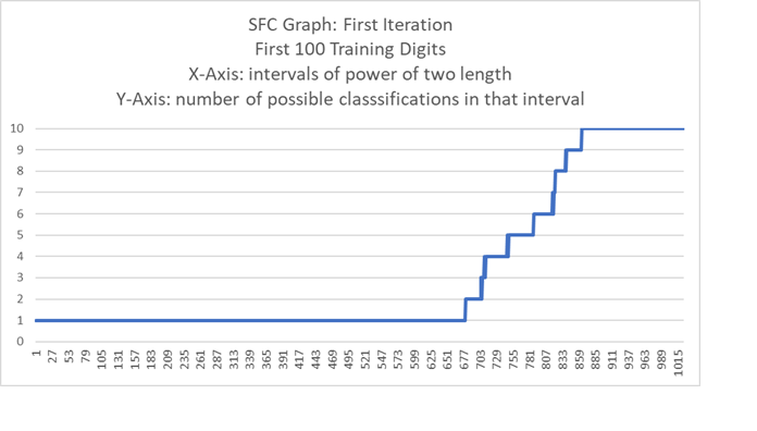
The following SFC graph uses the first 100 training digits (out of 60,000).
Using more training digits does not change the graph much since this is only the first iteration.
Each used pixel is a set bit in the binary vector which is gray code labeled vGray.
The key for the SFC map is the gray code converted to base two and labeled vBase2. This is the X-axis.
The classification of vGray or the grid is a digit between [0,9] and is on the Y-axis.
The first iteration is the same as all possible grids with only one bit set.
There are 1024 vGray vectors with one bit set.
The first iteration map of the SFC is of size 1024. C(1024,1) + 1 = 1024 (the plus 1 is from iteration zero or the origin, C(1024,0) = 1)
Each interval is a power of 2 long.
Each interval is as long as the sum of the lengths of all the previous intervals.
The maximum length of the SFC (X-axis) is 2^1024 long.
Since this is too big to graph, the X-axis is divided into intervals.
Each interval is an iteration with the lower bound equal to a map value and the upper bound just less than an upper (often but not necessarily next) value.
Each interval (X-axis) is classified (Y-axis) as all digits possible in that interval.
This calculation involves all training digits (points). It is not necessary to check all possible test digits (points) in all possible iterations of that interval.
The calculations are provided in the code.
The calculations took 30.745 seconds.
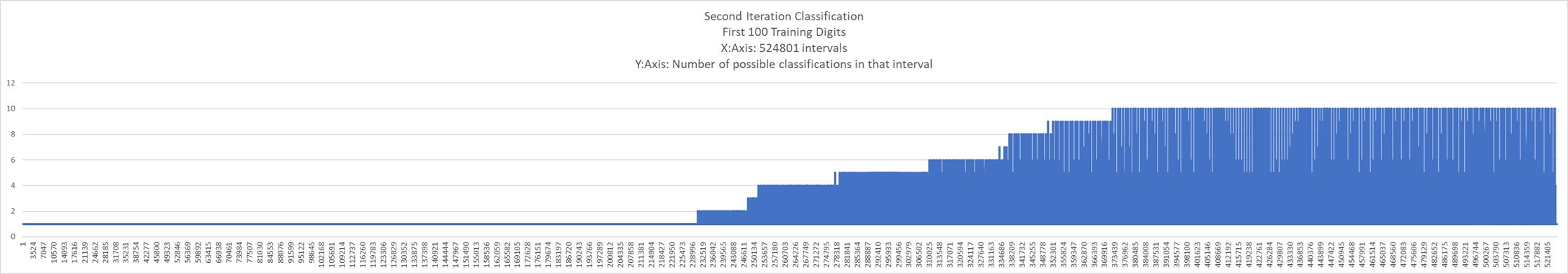
Iterating SFC Intervals with HWD: The Second Iteration (for this example there is a maximum of 1024 iterations)
The second iteration map of the SFC is of size C(1024,2) = 523776
The SFC map size for both iterations is C(1024,2) + C(1024,1) + C(1024,0) = 532776 + 1024 + 1 = 524801
The an iteration size with m total bits and n gray set bits is C(m,n).
The total length of the SFC or size of the map is 2^1024. That is also the number of possible test digits.
At its limit, the map of intervals becomes a map of points.
To generate the first iteration took .002 seconds.
To generate the second iteration took 7.015 seconds.
To calculate the classifications of the 524801 intervals took 4.36406 hours.
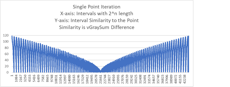
Iterating and Classifying to a Single Point (Note: Classifying takes the curve to 0)
Below is a graph of the iterations to a single random training point (digit) using a 28x28 = 784 pixel grid.
There are 117 iterations which produced 43303 intervals each of a power of two length.
The interval length at the point is 1.
The similarity is the vGraySum difference or XOR between the X-axis and the training point.
Time to iterate and classify the point is 1.793 seconds.
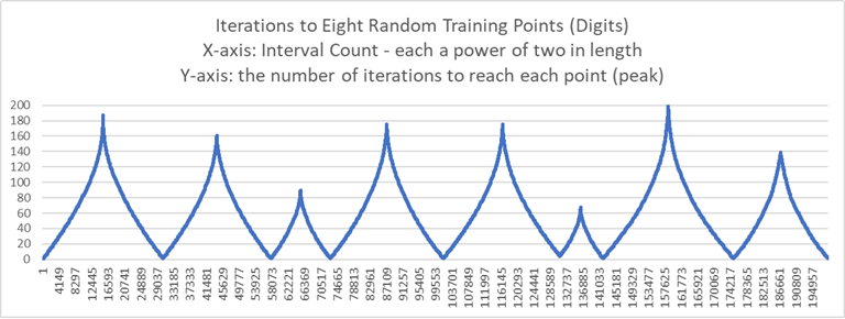
Iterating to a Eight Points (Note: Only Iterating and not Classifying takes the curve to the max nGraySum or max gray bits set)
The X-axis is the length of the SFC.
The Y-axis is the nGraySum or gray bits set. The nGraySum is equal to the number of iterations to reach that point.
The next graph iterates to eight random training points (digits) using a 28x28 = 784 pixel grid.
The unused pixels are removed leaving 341 pixels.
There are 199073 intervals which took 24.974 seconds to classify.
The previous graph showed the minimum nGraySum within an interval.
This graph shows the number of iterations for each interval with the peaks the number of iterations to reach a point (peak).
The number of iterations to reach a point (vector, digit) is equal to its nGraySum or number of gray bits set.
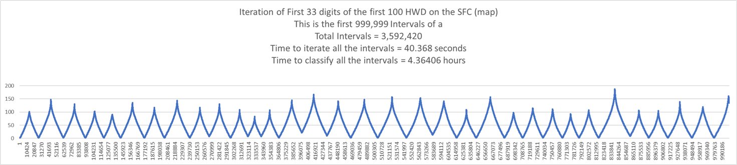
Iterating First 100 of the HWD (Graphing only the first 33)
The X-axis is the length of the SFC.
The Y-axis is the nGraySum or gray bits set.
There is very little overlap demonstrating there are many possible intervals between these intervals.
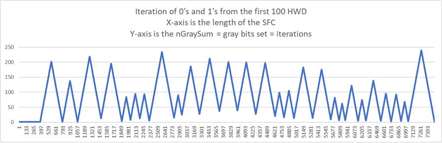
Graphing Digits: Digits Zero and One from the First 100 of the HWD Training Set
There are 27 digits. 13 are digit zero. 14 are digit one.
The next graph is the iteration of those 27 digits.
The X-axis is the length of the SFC.
The Y-axis is the nGraySum == gray bits set == iterations.
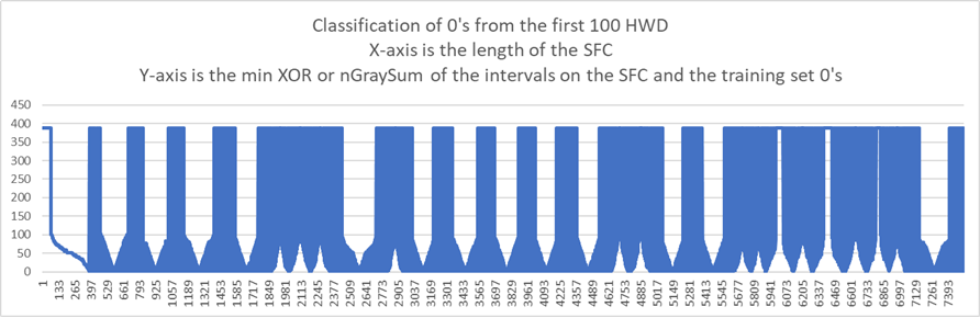
The next graph is the classification of the 13 zero digits.
The X-axis is the length of the SFC.
The Y-axis is the minimum XOR between the intervals on the SFC and the 0's from the training set.
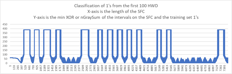
The next graph is the classification of the 14 one digits.
The X-axis is the length of the SFC.
The Y-axis is the minimum XOR between the intervals on the SFC and the 1's from the training set.
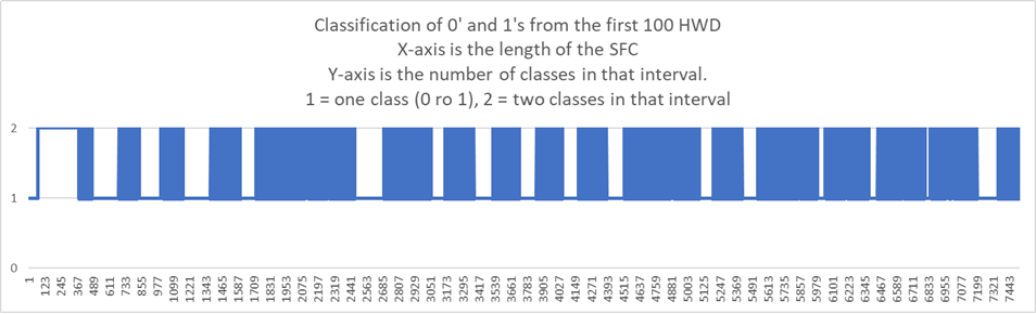
The next graph is the number of classifications in each interval on the SFC.
The X-axis is the length of the SFC.
The Y-axis is the number of classes in that interval. 1 = one class, 2 = two classes. In the case there is one class it may be a 0 or 1.
Classifying Iterative Intervals
By their nature, most SFC are non-differentiable or pointy everywhere. Poetically, the term for non-differentiability is fractal.
This allows the curve to get into every nook and cranny while every point on the curve has a limit in the space.
This property makes the above graphs move from one classification to another and back.
Consider test digits with a single positive pixel.
Using XOR as the measure of similarity, they always match with the training digit with the least pixels.
Next consider test digits with the same number of positive pixels.
These test digits have the same nGraySum and gray bits set and iteration.
For the HWD there is a maximum of 2^784 test digits but only 784 possible nGraySums or gray bits set or iterations given a single interval.
It is not necessary to use a single interval as the SFC may be divided into many intervals each with its own C(m,n) of nGrayBits, gray bits set, or iteration.
The following graphs use the same 0's and 1's from the first 100 of the HWD training set.
nGraySum == gray bits set == iteration = 100 is illustrative.
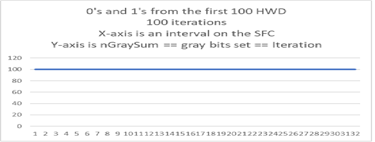
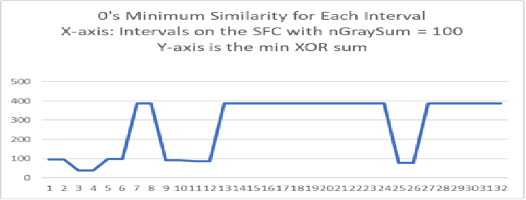
The next graph is the classification of the 13 zero digits.
The X-axis are intervals of the SFC such that all points in the interval have nGraySum = 100.
The Y-axis is the minimum XOR between the intervals on the SFC and the 0's from the training set.
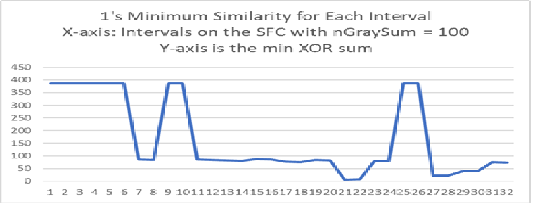
The next graph is the classification of the 14 one digits.
The X-axis are intervals of the SFC such that all points in the interval have nGraySum = 100.
The Y-axis is the minimum XOR between the intervals on the SFC and the 1's from the training set.
The next graph is the number of classifications in each interval on the SFC using digits 0,1.
The X-axis are intervals of the SFC such that all points in the interval have nGraySum = 100.
The Y-axis is the number of classes in that interval. 1 = one class, 2 = two classes. In the case there is one class it may be a 0 or 1.
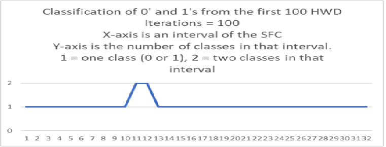
In the above case where there are two classes, their similarity is equal or differ by one.
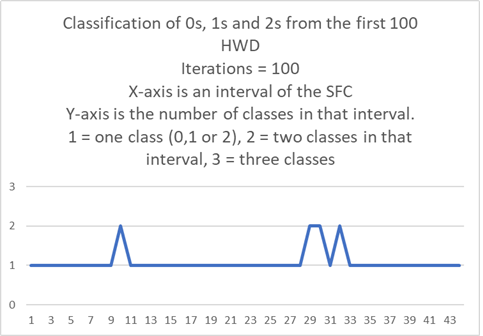
The next graph is the number of classifications in each interval on the SFC using digits 0,1,2.
The X-axis are intervals of the SFC such that all points in the interval have nGraySum = 100.
The Y-axis is the number of classes in that interval. 1 = one class, 2 = two classes 3 = three classes of which there are none here. In the case there is one class it may be a 0, 1, or 2.
Where there are two classes, their similarity differ by at most two.
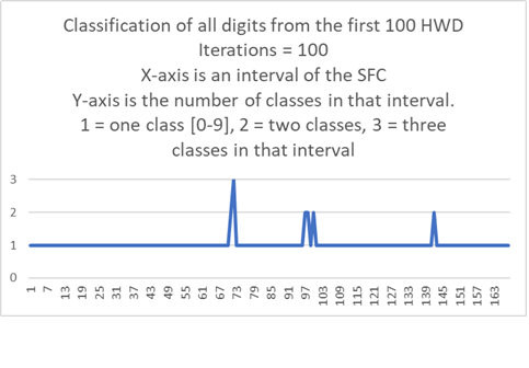
The next graph is the number of classifications in each interval on the SFC using all ten digits from the first 100 HWD.
The X-axis are intervals of the SFC such that all points in the interval have nGraySum = gray bits set = iterations = 100.
For these digits the max nGraySum = max gray bits set = max iterations = 240 so there are 240 of these graphs even though there are 501 pixels (out of 784) in use.
The Y-axis is the number of classes in that interval. 1 = one class, 2 = two classes, 3 = three classes.
There are none with four or more classes.
In the case where there is one class it may be any class.
Where there is more than one class, the similarities differ by at most two.
Redone to here.
5/11/2026
Knowledge Maps Using Supervised Learning:
Many of the examples here use hand written digits from zero to nine.
A point on the X-axis is a digit. The Y-axis is the classification (class) or type of digit.
There are many ways to write a digit but only ten possible classes for that digit yet the map is one-to-one.
Every point on the curve (X-axis) is mapped to (has) unique pixels and the classification(s) of those pixels.
Different measures of similarity generate different class clusters.
The following do not depend on the measure of similarity:
Given a training set and any two points on the SFC (X-axis) it is possible to calculate all possible classes between those two points.
Given a training set and any two points on the SFC (X-axis) and any range of combinations of binary pixels, it is possible to calculate all possible classes between those two points.
Given a training set and any point on the curve (X-axis), it is possible to generate every iterative step in its classification.
Format:
The points on the X-axis are vectors with element type bool. The size of these vectors is variable though here often 1024.
These points are labeled vBase2 since they represent a base two number and are keys for the map representing the curve.
When a vBase2 vector is converted to gray code, which is a vector of the same size and element type, it is labeled vGray.
For a gray code vector, the number of positive bits or bits set, (bits set to 1) is called the nGraySum.
This terminology is used because the bits set is usually different for vBase2 and vGray.
The nGraySum for vBase2 means vBase2 has been converted to gray code and then the bits summed.
The Hand Written Digits (HWD) come in a 28x28 = 784 bit grid but here 32x32 = 1024 is used.
GrayCode Example: void GrayCodeExample() in SFCMain2026.cpp
The key/curve is Base2. The value/data is gray code classified.
Since the curve is one-to-one, the value/data can be mapped one-to-one to the key.
A classification of the gray code is a point on the curve.
Note: Reordering the gray code reorders the map and classifications.
vBase2 and vGray Example .
Hilbert SFC Example: void HilbertCurveExample() in SFCMain2026.cpp
This curve has three dimensions and three bits per dimension.
Hilbert SFC Example.
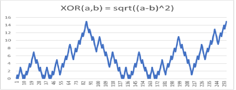
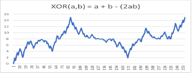
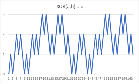
XOR Example: void XORExample() in SFCMain2026.cpp
XOR(a,b) = c
This curve has two dimensions and three bits per dimension.
XOR Example Data .
XOR Example Graph
Iterate Points Example: void IteratePointsExample() in SFCMain2026.cpp
Pick a point on the X-axis or key from the curve map. Make that vBase2 point the lower_bound.
Even though that point is a vBase2, it has a nGraySum.
Using the lower_bound, get the next point on the curve with the same nGraySum using GrayCode::IncrementBase2SameGraySum(lower_bound).
Make that vBase2 point the upper_bound.
Using the lower_bound, get the next point on the curve with the same nGraySum + 1 using GrayCode::IncrementBase2IncrementGraySum(lower_bound).
That first vBase2 point witb nGraySum + 1 is less than the upper_bound.
Using each next GrayCode::IncrementBase2SameGraySum(vBase2 with nGraySum + 1) continue until the upper_bound.
This is the function Intervals::IteratePoint generating a curve interval by iterating points.
Iterate Points Example .
Iterate to a Point Example: void IterateToPointExample() in SFCMain2026.cpp
This shows the iterations to a point. Code is also at Intervals::IterateToPoint.
The initial iteration map is the first calculation.
The lower_bound of the point is found in that map.
The point preceding the lower_bound is iterated until the point is reached.
The number of iterations is equal to the nGraySum of the point.
Iterate to Point Example .
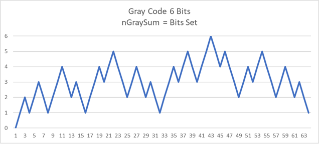
A graph of gray code nGraySum (gray bits set) using six bits.
C(6,3) = 20 is the maximum number of intervals between two points on a SFC.
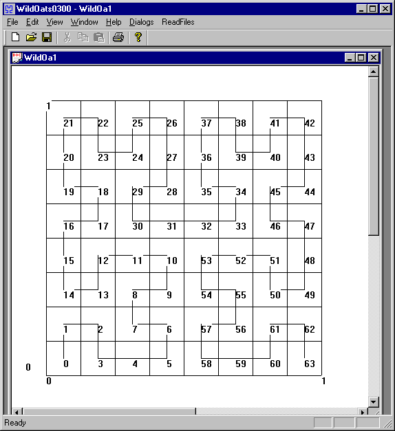
The Problem with this Approach
On the graph below, the points 10 and 53 are close as the crow flies but far as the curve crawls. However:
(Point#, nGraySum) Note: nGraySum = gray bits set
(10, 2)
(31, 3)
(32, 4)
(53, 3)
HWD Training Set first 100, SFC first iteration
The following graph is the SFC first iteration (size = 1025) classified with the first 100 training digits.
The pixels are ordered by frequency with the highest frequency of use to the left.
The X-axis has 1024 intervals.
Each interval has an increasing power of two length (size) which cannot be shown but can be iterated.
The total length (size) of the SFC and X-axis is 2^1024 which cannot be shown but can be iterated.
The next interval length is one more than the sum of all the previous interval lengths.
The next interval in gray code can be generated by reversing the order (reversing the ordering of the keys in a map) of all previous and adding a set bit to the left.
The next interval classification approximation is a reverse ordering of all the previous.
The Y-axis is the number of possible classifications in an interval. The number of intervals matter. The length (size) of the interval does not matter.
The number of intervals matter. The length (size) of the interval does not matter.
The time to generate the possible classifications in an interval depends on the size of the training set, not the size of the interval.
The following is for the first iteration.
For a training set size of 100, the time to generate graph: 0.546 minutes.
For a training set size of 200, the time was 2.192 minutes.
For a training set size of 500, the time was 13.626 minutes.
For a training set size of 1000, the time was 54.378 minutes.
There is there is the expected difference in the data (lower minimums, different indexes) while the graph of the classes is similar for the first iteration, regardless the training set size.
For this method and first iteration, most of the training points (digits) do not determine the classification.
Below is the output of the first iteration from which the graph was generated.
Each column is for a class of digit.
Each row is an interval on the space-filling curve. Each interval is a power(the first column) of two in length.
The first column is the power of two for that interval.
The first set of ten columns is the minimal nGraySum (gray bits set) possible in that interval. The number 1025 is off scale high.
The second set of ten columns is the index of the best possible training digit. The number 100 is off scale high.
The third set of ten columns is the classifications for that of the training digit. The number 10 is off scale high.
The last column is the number of possible classifications in that interval which was used to generate the graph.
SFC Iteration1 Training Set 100 text
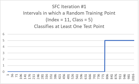
HWD Training Set first 100, SFC first iteration, Random Train Point(digit) with Index = 11 and Class = 5
The graph shows all possible intervals (one iterations) where a point (digit) will have a min nGraySum (gray bits set) with the Training Point (11,5).
Time to generate graph: 0.3 seconds.
Below is a point from an interval on the SFC.
Of all the training points, the best similarity is to the training point next below.
Bounded Interval Point MinSum = 96
00000000000000000000000000000000
00000000000000000000000000000000
00000000000000000000000000000000
00000000000000000000000000000000
00000000000000000000000000000000
00000000000000000000000000000000
00000000000000000000000000000000
00000000000000000000000000000000
00000000000000000000000000000000
00000000000000000000000000000000
00000000000000000000000100000000
00000000000000000000000100000000
00000000000100000000000100000000
00000000011100000000000100000000
00000000111100000000001100000000
00000000111000000000001000000000
00000000000000000000000000000000
00000000000000000000000000000000
00000000000000000000000000000000
00000000000000000000000000000000
00000000000000000000000000000000
00000000000000000000000000000000
00000000000000000000000000000000
00000000000000000000000000000000
00000000000000000000000000000000
00000000001000000000000000000000
00000000011110000000000000000000
00000000011110000000000000000000
00000000111100000000000000000000
00000000111000000000000000000000
00000000000000000000000000000000
00000000000000000000000000000000
This is the random training point with min nGraySum (gray bits set) = 96 to the above point.
The MinSum is an XOR derived value. Any measure of similarity will work.
Though different measuring sticks give different classifications at the edges.
Train Point (71, 7)
00000000000000000000000000000000
00000000000000000000000000000000
00000000000000000000000000000000
00000000000000000000000000000000
00000000000000000000000000000000
00000000000000000000000000000000
00000000000000000000000000000000
00000000000000000000000000000000
00000000000000000000000000000000
00000000000000000000000000000000
00000000000000011111111100000000
00000000000001111111111100000000
00000000000111111111111100000000
00000000011111111101111100000000
00000000111111111001111100000000
00000000111111100011111000000000
00000000000000000111110000000000
00000000000000001111100000000000
00000000000000001111000000000000
00000000000000011110000000000000
00000000000000111100000000000000
00000000000001111000000000000000
00000000000011110000000000000000
00000000000011110000000000000000
00000000000111100000000000000000
00000000001111000000000000000000
00000000011110000000000000000000
00000000011110000000000000000000
00000000111100000000000000000000
00000000111000000000000000000000
00000000000000000000000000000000
00000000000000000000000000000000
A Problem with this Method
For any point (digit), if the first gray bit is flipped, the two points are on different halves of the SFC.
As the crow flies, the two points are separated by one bit.
As the curve crawls, the two points might be separated by a zillion bits.
Select any two training points (digits).
Using both points, count how often each pixel, of the possible pixels, is used.
For two points, there are three possibilities, 0, 1, 2.
Select one point and make it the origin by XOR with itself and the other point.
The pixels with count 0 or 2 are now 0.
The pixels with count 1 remain 1.
This is an nGraySum or gray bits set.
Reorder all the pixels so the pixels with count 1 are all to the right. (It is not necessary to do this reorder but it makes it easier to see.)
For any point on the SFC (any test point), only the pixels, after the above transformations, with count 1 have any effect.
For any point on the SFC with less than half of that nGraySum, it is most similar to the origin.
For any point on the SFC with more than half of that nGraySum, it is most similar to the other point.
For any point on the SFC with equal to half of that nGraySum, it is most similar to both points.
A SFC graph classifying all possible test points for those two training points depends only on that nGraySum (gray bits set).
The code below needs revision.
XOR as a classifier is nearest neighbor with binary dimensions.
Classifying an Interval on the Curve
Any interval on the curve has a lower_bound and an upper_bound.
The classification includes the lower_bound up to but not including the upper_bound.
Classify the lower_bound.
Starting left with the most significant elements of each bound, select the elements that are all equal between the two boundaries.
For each training point (digit), make those are the left most elements.
Classify each modified training point to classify the interval.
This function is at Intervals::CalculateIntervalClassesAllSums.
Classifying an Interval on the Curve within nGraySum limits
Any interval on the curve may have nGraySum limits as opposed to the above which includes all possible sums.
This allows combinations of sums in any interval.
For any point on the curve, its elements are divided into sections.
The sections have sum lower and upper limits which in turn limits the possible classifications.
Given any section, starting on the right, gray bits of a training point are flipped to place the section within the limits.
Then that point is classified.
This function is at Intervals::CalculateIntervalClassesSameSums. Note: this may over classify (include extra classes) for low iterations.
Classifying a Point on the Curve
For this prototype, XOR is the classifier.
Handwritten Digits are used for the training and test sets.
A digit’s pixels are read as gray code.
The pixels are in [0,255]. Any number greater than zero is set to one making the pixels binary.
Fuzzy pixels do not seem to be an improvement with these methods at this time.
A test point gray code is XOR with each training set gray code.
The minimum nGraySum of the result is the measure of similarity.
This is similar to nearest neighbor.
This function is at MeasureOfSimilarity::XORPointClassification.
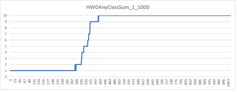
Classifying the Entire Curve Using all Combinations of Pixels is Typically not Practical
The graph below shows the first iteration of the first 1000 digits.
The X-axis is an interval with an increasing power of two length. The total length is 2^1024.
The Y-axis is the number of classifications in each interval.
Every interval with more than one classification usually needs an additional iteration.
Though the iterative limit of any point is the nGraySum of that point, the number of iterative points grows exponential.
While it is possible to limit the growth by limiting the nGraySum in any interval, this is not appealing and often not practical.
The best option seems to be the selection of intervals with undesirable classifications for additional iterations then studying their inputs.
Evaluating Test Points
After the curve (map) is generated, a test point has a lower_bound. That lower bound is the classification.
If there is more than one possible classification in that interval, the test point is iterated until it is classified.
Fuzzy Pixels
If instead of binary pixels, fuzzy pixels are desired, the Hilbert Curve is used. The example and code is referenced above.
For HWD if would have 28x28 = 784 dimensions with 8 bits per dimension. Total bits per point 784 x 8 = 6272. Length of the curve = 2 ^ 6272.
XOR would not be used as the measure of similarity.
Finding the Axioms
For HWD the axioms are the training set. These can be found since their measure of similarity is zero in this setting.
If a training point is always bounded by another of the same class, that training point could be removed.
The C++ code
Gray Code
GrayCode.h
GrayCode.cpp
Intervals
Intervals are segments of the curve.
An interval starts with its first point and ends just prior to the next interval.
All possible classifications within an interval can be calculated.
The calculation for each interval depends on the size of the training set and the size of each point.
The calculation for each interval does not depend on the size of the interval or curve.
Interval classifications may be restricted to combinations of Gray Sums (the sum of gray code ones).
Intervals.h
Intervals.cpp
Measure of Similarity
For now, XOR is the measure of similarity because this is a prototype and XOR is fast and simple.
It is possible that at a future time, a neural network can be placed, with modifications throughout, in this vicinity.
XOR is applied to the gray code, which is the data, and is equivalent to nearest neighbor for binary pixels.
Curiously, for Hand Written Digits, it appears XOR is more accurate than fuzzy pixels and nearest neighbor.
MeasureOfSimilarity.h
MeasureOfSimilarity.cpp
Hand Written Digits
My Hand Written Digits dataset is decades old and here is the old link:
The MNIST database of handwritten digits
This looks similiar to what I am using.
Here is my code to show my work but I doubt anyone will use mine.
The digits are in a 28x28 grid of pixels. For my program, I change the grid to 32x32 in GrayCode.cpp to make it easier to manipulate the intervals.
The above step does not add much time to the calculations.
HandWrittenDigits.h
HandWrittenDigits.cpp
Input/Output
IO.h
IO.cpp
This is where I run my program. It is in flux.
It uses the year 2026 as an aspiration.
SFCMain2026.cpp
My Hardware:
Processor: AMD Ryzen 7 5800X 8-Core Processor, 3801 Mhz, 8 Core(s), 16 Logical Processor(s)
The graphics card is not used for these calculations.
I might be making slow progress translating some physics equations to the same thing but from a space-filling curve perspective.
I will send you some thoughts for correction when I get more comfortable.
The idea is that no one knows what a number is, only what the properties of numbers are.
Physics is the same way. Nothing new here. Just a method for me to understand physics better.
It seems curious the equations for quantum physics are often differential or smooth. Quantum means non-differential or pointy.
What would physics look like through the lens of non-differential mathematics?
This would not change much except our understanding and perhaps an epsilon of a chance to harvest the quantum vacuum while we sail within it.
For instance, the energy of a photon is E = hf. E is the energy, h is a constant, f is the frequency.
Frequency is an oscillator which implies the energy oscillates which is false.
A photon also has a wave-length. Waves are differentiable or smooth.
Suppose that instead of a particle-wave duality, the photon is a space-filling curve (SFC).
Its frequency could be the iteration, the wave-length the length of the curve, and its amplitude the size of the SFC.
This probably goes nowhere.
In any case, that is the start of Phase II.
Sagan, H. 1994
Space-Filling Curves
NY, NY.:Springer-Verlag.
ISBN 0-387-94265-3
Best reference for space-filling curves.
On the back cover:
"Cantor showed in 1878 that there is a one-to-one correspondence
between an interval and a square (or cube, or any finite-dimensional
manifold) and Netto demonstrated that such a correspondence
cannot be continuous. Dropping the requirement that the mapping
be one-to-one, Peano found a continuous map from the interval onto
the square (or cube) in 1890. In other words: He found a continuous
curve that passes through every point of the square (or cube).
This book discusses generalizations and modifications of Peano's
constructions, the properties of such curves, and their relationship to fractals."
Peitgen, H., Jurgens, H., and Saupe, D., 1992
Chaos and Fractals
NY,NY.: Springer-Verlag.
ISBN 3-540-97903-4
Nice place to start.
Chaos is a poetic term for recursiveness or self-referencing.
Fractal is a poetic term for being non-differentiable (pointy).
Spivak, Michael 1967
Calculus
W. A. Benjamin, Inc
ISBN 978-0-914098-91-1
An Introduction to functions.
The best book I have ever read.
Bell, J.L., Slomson, A.B. 1969
Models and Ultraproducts
North-Holland Publishing Company
Library of Congress Catalog Card Number: 78-87273
An Introduction to logic.
Milonni, P. 1994
The Quantum Vacuum
Academic Press
ISBN 0-12-498080-5
An empty vacuum does not exist.
Site posted:
11/01/1999 as medicalautopilot.com
12/2020 as MedicalAutopilot.net - Healthcare Reform and a Medical Autopilot(perhaps)
12/2021 as spacefilligcurve.com
Last modified: June/2024
Here is a bit on Philosophy
My email address is the first two initials, last name at comcast dot net
I am a retired general/trauma surgeon.
Surgery is a fabulous profession. Five stars – highly recommended – would do it again.
James J. Rice